Software & code
SDMs with alpha-shapes | Kappa calculator | Raster ASCII to single vector
R code for predicting species potential distributions using Alpha-shapes
Alpha-shapes have several interesting properties to predict distributions in new areas (e.g. an invasive species) or time periods (e.g. range changes under climate change). For instance they only require presence data, they fit flexible environmental envelopes and the realism of the fitted envelope can be easily assessed visually. You can read more about this method in our recent paper in Ecological Informatics.
In this example I’ll use data for the Gold-striped salamander (Chioglossa lusitanica), a species confined to the Northwest of the Iberian Peninsula. Distribution data comes from the “Inventario Español de Especies Terrestres” and the “Atlas dos Anfíbios e Répteis de Portugal”. I will use alpha-shapes for predicting the species' current range and its potential range in 2041–2060 under the climate predicted for the greenhouse gas emissions scenario A2 (please see this other paper for details on the climate data). You can download the datasets here.
This example requires the use of the “alphashape3d” and the “raster” libraries.
library(alphashape3d)
library(raster)
Next it is advisable to define a working directory in which all datasets are stored, I’ll use “D://C_lusitanica” in this example.
setwd("D://C_lusitanica")
In this folder there should be one “.csv” file containing the longitude and latitude of each of the species occurrences as well as all current climatic datasets in raster ASCII format. Finally there should also be a separate folder or subfolder containing the future climate datasets (in this case a subfolder named: “future_climate_A2”). These future climate datasets should have the same filenames than those of current climate.
#Load occurrence data
occur.data <- read.table("occ_C_lusitanica.csv", header=TRUE, sep=",", na.strings="NA", dec=".")
#Load climatic predictors
grids <- list.files(pattern='asc', full.names=T) #Loads all “.asc” files in folder
predictors <- stack(grids) #Make a “stack” of current climate layers
grids.future<- list.files(path = "D://C_lusitanica//future_climate_A2", pattern='asc', full.names=T) #Loads all future climate “.asc” files in folder
predictors.future <- stack(grids.future) #Make a “stack” of future climate layers
Alpha-shapes can only be computed in two or three dimensions. In other words we can only consider two or three predictors; this sounds like a bugger (and sometimes it is) but in many cases it can also be a desirable property because it ensures an intuitive and transparent model (see discussion in our paper). Here I considered five climatic predictors (mean diurnal range; mean maximum temperature of the warmest month; mean minimum temperature of the coldest month; mean yearly total rainfall and mean) and in order to comply with the low-dimensionality requirements of alpha-shapes we’ll use a principal components analysis to extract the three main axes.
pca <- princomp(na.omit(values(predictors)), cor=TRUE) #Compute a PCA
PCs <- predict(predictors, pca, index=1:3) #Extract the scores of the three first axes of the PCA
occur.PCs <- extract(PCs, occur.data) #Extract the scores of the three axes for each occurrence record
PCs.points <- rasterToPoints(PCs) #Convert cells of raster PCA axes to points
Optionally, we can visualize the species occurrences in the 3D climatic space.
plot3d(occur.PCs, col = 'blue', type = 's' ,size=0.5)
Next, we will identify the minimum bounding envelope of this point set. Note that the MBE is an envelope that is tightly adjusted to the species occurrences and sometimes other bounding criteria may be preferable (e.g. when the number of occurrences is very limited). The minimum bounding envelope (MBE) corresponds to the envelope that captures all occurrence records and has no hollow spaces. To identify the MBE, it is necessary to evaluate distinct values of alpha (the radius of an imaginary sphere that is used to define the inclusion or exclusion of neighboring occurrences). To that end we compute alpha-shapes with continuously increasing values of alpha and test which is the first to enclose all species occurrences.
i<-seq(0, 2, by = 0.01) #Define the value of alpha for which each alpha-shape will be computed.
ashape3d.occ <- ashape3d(unique(as.matrix(occur.PCs)), alpha = i) #Compute the alpha-shape.
result.occurrence <- inashape3d(ashape3d.occ, indexAlpha="all", points = as.matrix(occur.PCs)) #Test if species occurrences are inside or outside the alpha-shape
percentage<-unlist(lapply(result.occurrence,"mean")) #Calculate the percentage of occurrences inside the alpha-shape.
values <-data.frame(i,percentage*100) #A data frame containing the percentage of occurrences included in each of the alpha-shapes.
By inspecting the vector “values” we verify that the first envelope to contain all occurrences is achieved at an alpha=1.19. We now compute this alpha-shape and inspect if it has any hollow spaces (e.g. “holes” or “voids”).
alpha <- 1.19 #Define the selected value of alpha.
ashape3d.occ <- ashape3d(unique(as.matrix(occur.PCs)), alpha = alpha) #Compute the alpha-shape for the selected value.
plot(ashape3d.occ,bycom=TRUE,tran=0.2,shininess=0) #Plot in search of hollow spaces.
rgl.bbox(color=c("#333377","white"), emission="#333377", specular="#3333FF", shininess=5, alpha=0.8 )

inside.occur.shape <- inashape3d(ashape3d.occ, points = PCs.points[,3:5])# Test if conditions are inside or outside the envelope.
occur.pred <- cbind(PCs.points[,1:2], inside.occur.shape) #Bind geographical coordinates with classification.
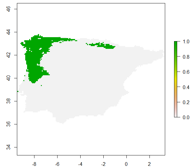
raster.result <- rasterize(x = occur.pred[,1:2], y = predictors[[1]], field = occur.pred[,3]) #Convert to raster format
plot(raster.result) #Visualize current potential range
PCs.future <- predict(predictors.future, pca, index=1:3) #Scores of the three first axes of the PCA
PCs.points.future <- rasterToPoints(PCs.future)
future.inside.occur.shape <- inashape3d(ashape3d.occ, points = PCs.points.future[,3:5])# Test if conditions are inside or outside the envelope.
future.occur.pred <- cbind(PCs.points.future [,1:2], future.inside.occur.shape) #Bind geographical coordinates with classification.
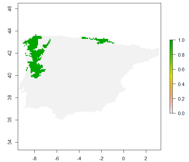
raster.result.future <- rasterize(x = future.occur.pred [,1:2], y = predictors[[1]], field = future.occur.pred [,3])#Convert to raster format.
plot(raster.result.future) #Visualize future potential range.
Kappa calculator

This is a small program I've made to help me on the multiple calculations of the kappa statistic along a predefined range of thresholds.
The required parameters are: lower value (ex. 0); higher value (ex. 1) and number thresholds. The threshold amplitude will be calculated as (higher value - lower value)/number of classes.
The lists of values are inputted as a plain text file with one column only (see example files). You must then provide a name for the text file that will store the results. This file will be automatically opened and in it you’ll have the threshold and the Kappa value for it.
Download
Raster ASCII to single vector
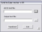
This a set of two tools. The first "Deconstruct" converts ASCII raster maps to a single column file. The "Reconstruct" tool rebuilds the column again as ASCII Raster. This tools can be usefull to perform statistical analysis outside the GIS software environments.
Notice: These tools are still not thoroughly tested, especially the "Reconstruct" tool which is very slow for large files.
Download ASCII Raster to single vector
Word Inverter 1.0

This is just a small funny utility which allows to invert the order of characters of a text.
Ex.: Hello -> olleH.

